Where do p-values come from? Fundamental concepts and simulation approach
tl;dr: P-values are tail probabilities calculated from the sampling distribution of a sample-based statistic. This sampling distribution will depend on the size of the sample, the statistic being calculated and assumptions about the random population from which the data could have been sampled. For a few cases, analytical p-values are available and, for the rest of cases, approximations based on Monte Carlo simulation can be computed by generating the sampling distribution from the population.
What is a p-value?
In order to understand what a p-value is and what it measures, we need to go deeper into the theory behind them (the figure below illustrates what is discussed in this article). P-values belong to an statistical paradigm known as frequentist statistics (this is what you were taught in high school and basic stats courses). When analysing data using this paradigm, one needs to assume a “hypothetical infinite population, of which the actual data are regarded as constituting a random sample” (Fisher, 1923). Whether that hypothetical population does exist or not is irrelevant, as the ultimate role of this random population is to facilitate making statements about phenomena in the presence of unexplained variance or noise. Of course, this approach is most useful when there is an actual population from which the data were sampled (or when individuals were randomly assigned to groups), as it becomes easier to find a proper distribution to describe the population.
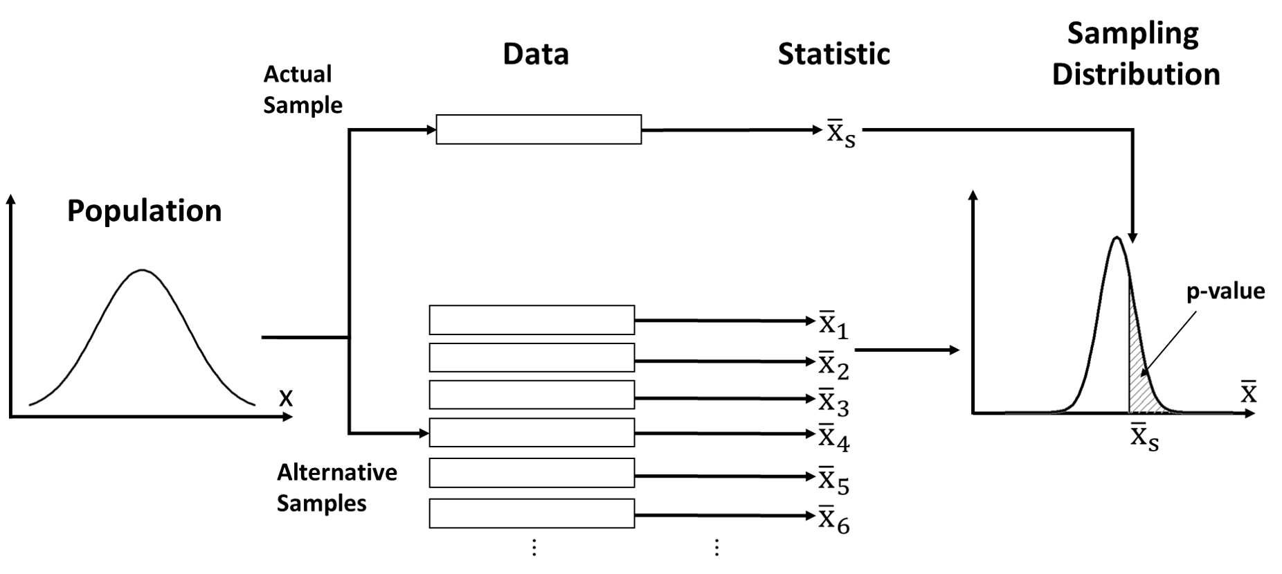
Since the data are interpreted as a random sample, any quantity calculated from the data (e.g. the arithmetic mean of observed values, \(\bar{x}\)) can be treated as a random variable. That is, each random sample from the population will yield a different value of the same quantity (e.g. different sample means). Also, it means that these quantities will follow a probability distribution. For example, if we take multiple random samples from the same population, and calculate the mean of each of these samples, some values of the sample mean will be more common that others. This distribution is what we call the sampling distribution and the quantity derived from samples is called statistic. In frequentist statistics, any probability statement (e.g. p-values, confidence intervals) always refers to a statistic and its associated sampling distribution.
The other important concept behind p-value is that of hypothesis testing. A null hypohtesis is a statement about differences between groups or phenomena. The null hypothesis represnets a default skeptical position (i.e. no difference). The goal of null hypothesis significant testing (NHST) is to challenge the null hypothesis given observed data. This procedure requires building a statistical model to describe the random population from which the data could have been sampled, assuming that the null hypothesis is true. Then, one calculates how likely it is for the observed data to occur assuming it was sampled from that population. The more unlikely the data are, the less likely the null hypothesis becomes. However, comparing the observed data to all possible alternative data is too difficult, so the problem is often simplified to comparing a statistic calculated from the data with all the possible values of the same statistic that could have been obtained from the population. In practice, this means that we need to construct a sampling distribution and evaluate how unlikely the observed statistic is within that sampling distribution.
The final complication is that the quantities that we use as statistic are often continuous measures of the data (even when the data is composed of discrete values) but the basic laws of probability tells us that the probability of any particular value of a continuous random variable is exactly zero (there are many resources online explaining this idea, for example, this one). Therefore, calculating the probability of a particular statistic value in a sampling distribution is futile. As alternative, one can calculate the probability of all values more extreme than the observed (i.e. the shaded area in the figure above). The smaller this probability, the more unlikely the value is. And this probability is the p-value!
Since all this was very abstract, we will go through a classic example: the one sample t-test. I will illustrate with a computational approach how the sampling distribution arises from the population and how it relates to the sample statistic. I chose R as the programming language for this article as this is a common language for statistics, but the same approach could have done in Matlab/Octave, Python or Julia.
Example for the one sample mean test (one sample t-test)
Let’s imagine that we have a small dataset such as:
sample = c(1.52, 5.24, -0.23, 2.47, 2.63)Most values are positive and we may want to test whether the underlying effect is indeed positive. We will assume that this data could be treated as a random sample from a Normal population with a positive mean (i.e. \(\mu > 0\)). As described above, we set as null hypothesis (\(H_0\)) the more conservative option, which in the case it would be \(\mu = 0\), while the contesting or alternative hypothesis (\(H_1\)) represents positive case (\(\mu > 0\)). Formally, this is written as:
\[ \begin{align} H_{0} &: \mu = \mu_0 \\ H_{1} &: \mu > \mu_0 \end{align} \]
Where \(\mu_0 = 0\) in this case. Assuming that the sampling procedure ensures statistical independence and given the assumptions in the above, we could use the t statistic, \((\bar{x} - \mu_0)/(s/\sqrt n )\), where \(\bar{x}\) is the sample mean, \(s\) is the standard deviation of the sample and \(n\) is the sample size. The reason for using this statistic is that the sampling distribution is known to be a Student’s t distribution. The proof for this was given by William Gosset in 1908 (signed with the pseudonym Student). If you want to check what it takes to make such a proof, take a look at the original paper.
Rather than going through the mathematical proof, I will use a simulation-based procedure that I find more intuitive and easier to follow, and it is also very general, while producing the same results. Effectively, we will construct a Monte Carlo approximation to the sampling distribution of the t statistic. The computational procedure is as follows:
Estimate all the parameters of the population from the sample, except for the parameter that is already fixed by the null hypothesis. In this example, this means that we estimate the standard deviation of the Normal population (\(\sigma\)) from the sample, while fixing the mean (\(\mu\)) to 0.
Generate \(N\) random samples from the population of size \(n\) using the Monte Carlo method. In this case \(n\) is equal to 5 and \(N\) can be as large as you want (the larger the better).
For each sample generated in step 2, calculate the statistic. In this this case, we calculate \((\bar{x} - \mu_0)/(s/\sqrt n )\) for each sample.
The \(N\) statistics calculated in step 3 is a large sample of values from the sampling distribution. The p-value can then be calculated as the fraction of this sample that exceeds (or is lower, depending on the tail being tested) than the value of the statistic in the actual data.
Technical intermezzo
To put into practice these ideas with R, we need to load a couple of libraries:
- furrr that facilitates parallel execution of code on multiple processes based on the package future, because life is too short to wait for computations.
- distr6 to create and manipulate probability distributions.
for(lib in c("furrr", "distr6")) {
  library(lib, character.only = TRUE)
}
To turn on parallel computation we need the following bit of code:
plan(multiprocess)Finally, to make sure that we always get the same output, we need to initialise the random number generator:
set.seed(2019)Estimating parameters of the population
There are differences methods to estimate the parameters of an statistical model or distribution from a sample. For the case of the standard deviation of a Normal distribution, the canonical approach is to use the standard deviation with Bessel’s correction, also know as sample standard deviation (i.e. using n - 1 rather than n). It turns out that this is the default behaviour for R’s sd function, so the estimator is simply:
sigma_hat = sd(sample)The other parameter of the Normal distribution is fixed by the null hypothesis:
mu = 0Constructing the sampling distribution
First, let’s build the Normal distribution that describes the population:
population = Normal$new(mean = mu, sd = sigma_hat)Next, we need a function that calculates the statistic \((\bar{x} - \mu_0)/(s/\sqrt n )\) for a given sample
calc_statistic = function(x, mu0 = 0) {
  (mean(x) - mu0)/(sd(x)/sqrt(length(x)))
}
Then, we generate \(N\) samples from the population and calculate the statistic for each of them. The larger \(N\) is, the more accurate the calculation of the p-value will be. It turns out that calculating accurate p-values is computationally hard so, to make sure that our calculations are accurate, let’s generate 50000 samples:
N = 5e4
sampling_distribution = future_map_dbl(1:N, ~ calc_statistic(population$rand(5)))
Let’s compare the sampling_distribution with the theoretical distribution and the observed sample statistic:
plot(density(sampling_distribution,), xlab = "t statistic", main = "", xlim = c(-10,10)) # Histogram of sampling_distribution
curve(dt(x,4), -10, 10, add = T, col = 2, n = 1e3) # Theoretical distribution t(n-1)
abline(v = calc_statistic(sample), col = 3) # Observed statistic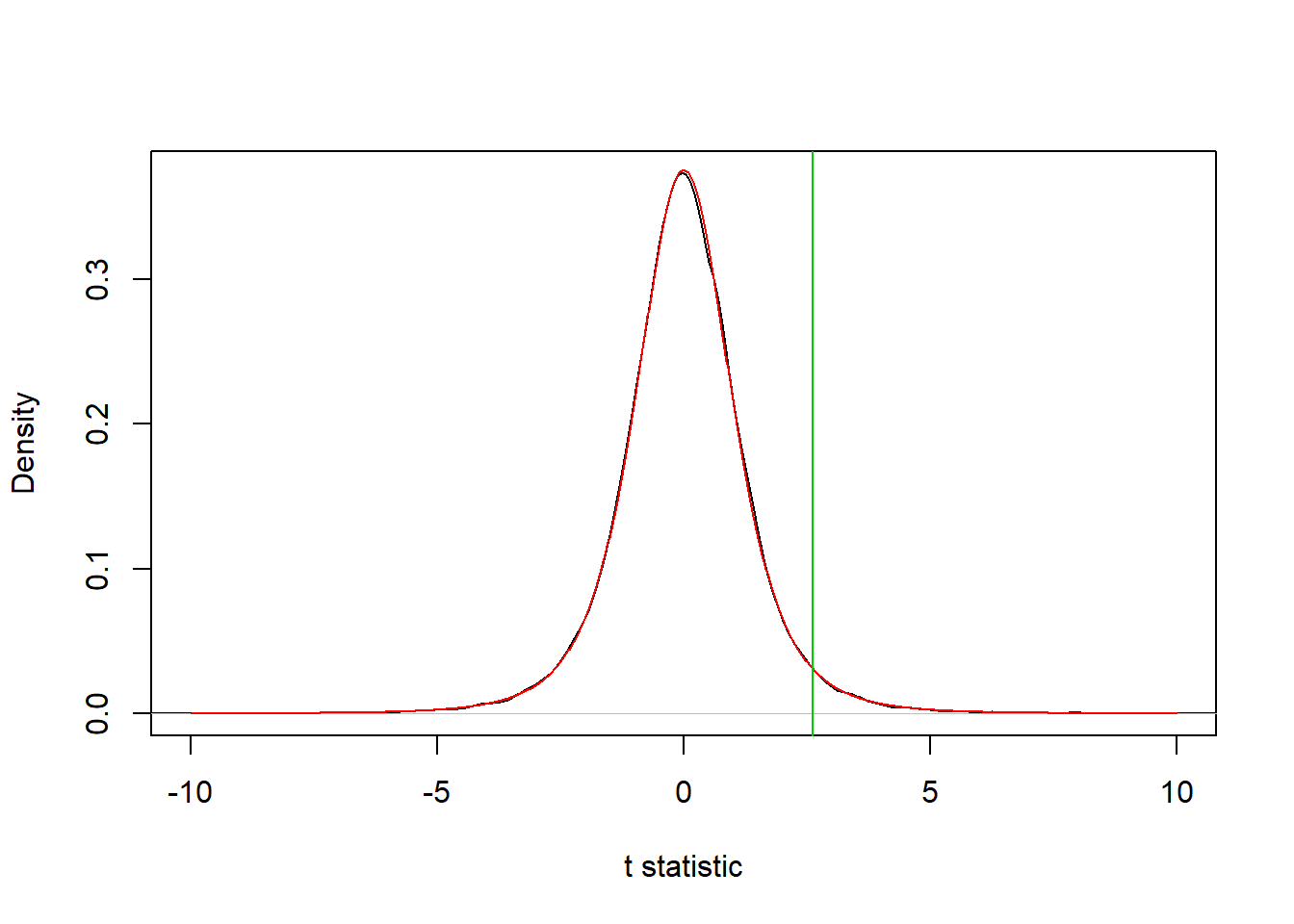
We can see that, indeed, the sampling distribution is Student’s t distribution with 4 degrees of freedom. Also, the observed value for the statistic is in an area of low probability in the sampling distribution, which suggest that this result may not be very likely to occur under the null hypothesis.
Calculate the p-value
In this example, the p-value is defined as the probability that a sample from the null hypothesis model leads to an statistic equal or larger than the observed one. Calculating this value from sampling distribution is as simple as computing the fraction of cases where this condition is met:
sum(sampling_distribution >= calc_statistic(sample))/N## [1] 0.02874We can compare this value from the one obtained from the t distribution:
1 - pt(calc_statistic(sample), 4)## [1] 0.02946129and with the results of calling the function t.test in R (which should be the same as for the t distribution unless I learnt the wrong theory…):
t.test(sample, alternative = "greater")$p.val## [1] 0.02946129We can see that the Monte Carlo estimate is very similar to the analytical value. Notice that there is still some small numerical error of about 3.7% despite the large number of Monte Carlo samples. There are more advanced methods to refine a Monte Carlo p-value estimate, but I will those for future posts.
Why not just use the sample mean as statistic?
Using the sample mean (\(\bar{x}\)) as statistic rather than \((\bar{x} - \mu_0)/(s/\sqrt n )\) would have been more intuitive, since we are asking a question about the mean, not some complicated function of it. With the simulation based approach this is trivial (or at least not more difficult than above). Let’s create the sampling distribution for the sample mean:
N = 5e4
sampling_distribution = future_map_dbl(1:N, ~ mean(population$rand(5)))
which looks like
plot(density(sampling_distribution, bw = "SJ"), main = "", xlab = "sample mean") # Histogram of sampling_distribution
abline(v = mean(sample), col = 2) # Observed statistic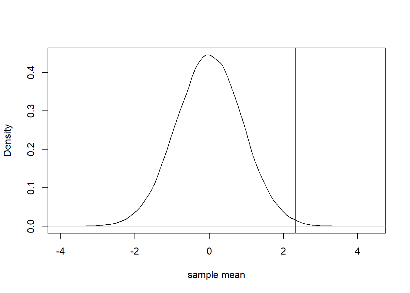
And the p-value is calculated in the same way as before:
sum(sampling_distribution >= mean(sample))/N## [1] 0.0043Notice that the p-value is different from the one before. This is not wrong, as given the same sample and population model, the p-value will depend on the statistic being calculated. You may me wondering what the analytical value would be in this case. As far as I know there is none, the reason being that so far it has not been possible to derive the sampling distribution for the sample mean. The only results known are for a hypothetical sample of infinite size (when the sampling distribution become Normal, regardless of the population). While these results may be used reasonably for large samples, it clearly does not apply for a sample size of 5.
Final remarks
As has been shown in this article, in order to calculate the p-value of an statistic we need to know its sampling distribution, which depends on the model assumed for the population. Traditionally, one had to derive the sampling distribution mathematically (if possible) for every combination of statistic and population model. This greatly restricts the number of scenarios which can be handled by traditional statistical tests, which leads to that dreaded question: “Which statistical test should I use for my data?”. There are dozens of decision trees that the practioner of statistics is supposed to follow (you can see some in this paper).
Nowadays, you can use a simulation approach such as the one presented in this article. With such an approach, you can always calculate the p-value for any statistic and population model, even if no one has ever tried that particular combination before. Restricting oneself to analytical methods made sense in the early 20th century when many of these tests were developed, but in the 21st century you can use computers! In the next post I will show how to apply this method to real world data that was not (and could not be) normally distributed. Stay tuned!