Maximum likelihood estimates of a distribution

Maximum likelihood estimation (MLE) is a method to estimate the parameters of a random population given a sample. I described what this population means and its relationship to the sample in a previous post.

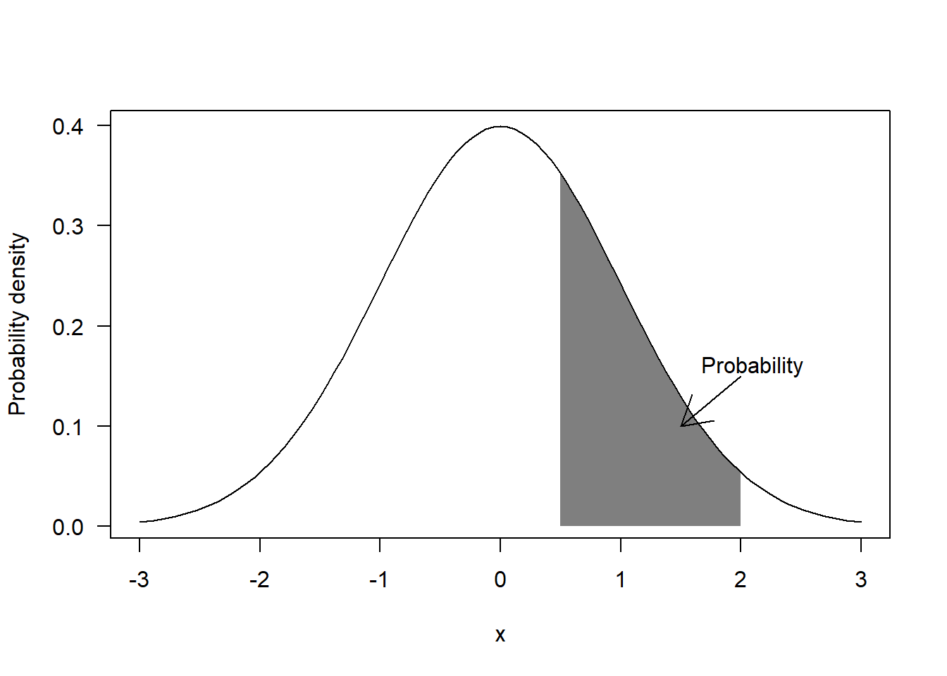
Before we can look into MLE, we first need to understand the difference between probability and probability density for continuous variables. Probability density can be seen as a measure of relative probability, that is, values located in areas with higher probability will get have higher probability density. More precisely, probability is the integral of probability density over a range. For example, the classic “bell-shaped” curve associated to the Normal distribution is a measure of probability density, whereas probability corresponds to the area under the curve for a given range of values:

If we assign an statistical model to the random population, any particular value (let’s call it \(x_i\)) sampled from the population will have a probability density according to the model (let’s call it \(f(x_i)\)). If we then assume that all the values in our sample are statistically independent (i.e. the probability of sampling a particular value does not depend on the rest of values already sampled), then the likelihood of observing the whole sample (let’s call it \(L(x)\)) is defined as the product of the probability densities of the individual values (i.e. \(L(x) = \prod_{i=1}^{i=n}f(x_i)\) where \(n\) is the size of the sample).

For example, if we assume that the data were sampled from a Normal distribution, the likelihood is defined as:

\[ L(x) = \prod_{i=1}^{i=n}\frac{1}{\sqrt{2 \pi \sigma^2}}e^{-\frac{\left(x_i - \mu \right)^2}{2\sigma^2}} \]

Note that \(L(x)\) does not depend on \(x\) only, but also on \(\mu\) and \(\sigma\), that is, the parameters in the statistical model describing the random population. The idea behind MLE is to find the values of the parameters in the statistical model that maximize \(L(x)\). In other words, it calculates the random population that is most likely to generate the observed data, while being constrained to a particular type of distribution.

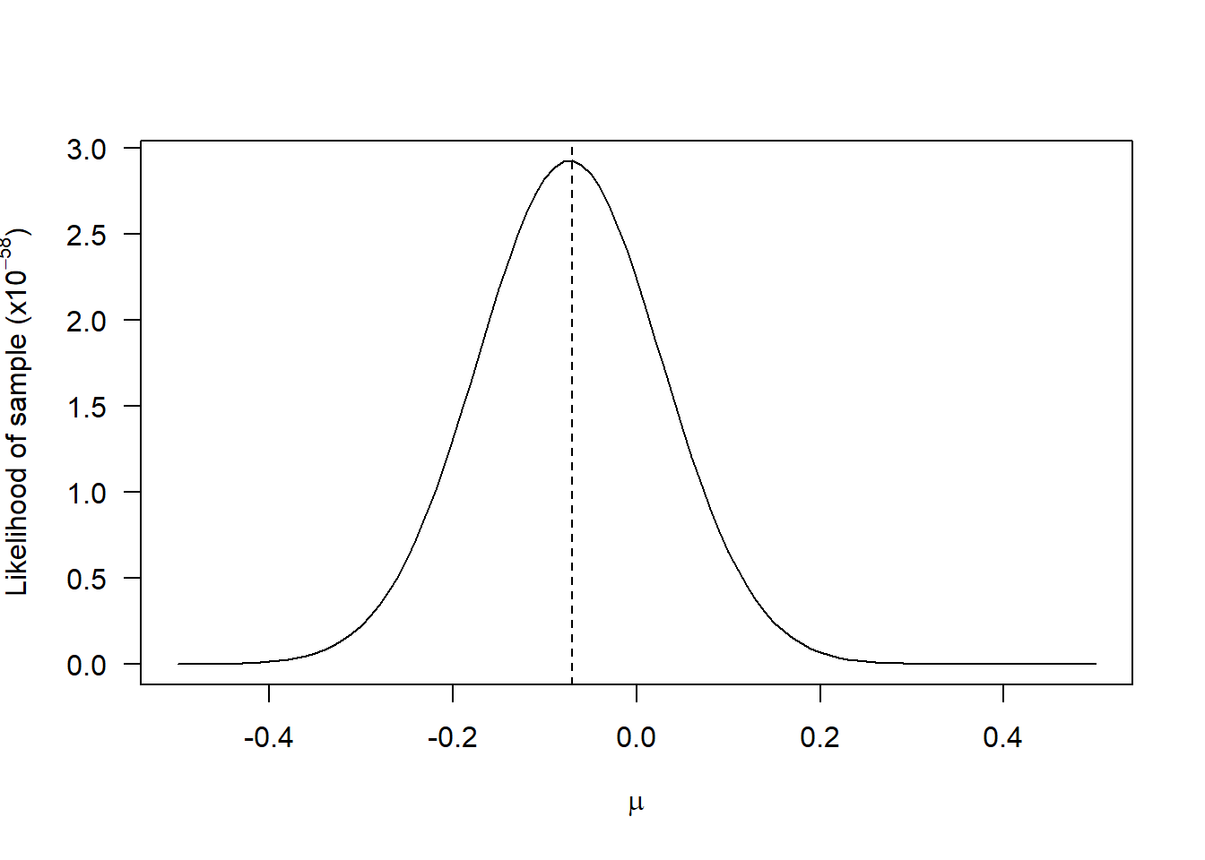
One complication of the MLE method is that, as probability densities are often smaller than 1, the value of \(L(x)\) can become very small as the sample size grows. For example the likelihood of 100 values sampled from a standard Normal distribution is very small:

set.seed(2019)
sample = rnorm(100)
prod(dnorm(sample))

## [1] 2.23626e-58

When the variance of the distribution is small it is also possible to have probability densities higher than one. In this case, the likelihood function will grow to very large values. For example, for a Normal distribution with standard deviation of 0.1 we get:

sample_large = rnorm(100, sd = 0.1)
prod(dnorm(sample_large, sd = 0.1))

## [1] 2.741535e+38

The reason why this is a problem is that computers have a limited capacity to store the digits of a number, so they cannot store very large or very small numbers. If you repeat the code above but using sample sizes of say 1000, you will get 0 or Inf instead of the actual values, because your computer will just give up. Although it is possible to increase the amount of digits to be stored per number, this does not really solve the problem, as it will eventually come back with larger samples. Furthermore, in most cases we will need to use numerical optimization algorithms (see below) which will make the problem even worse. Therefore, we cannot work directly with the likelihood function.

One trick is to use the natural logarithm of the likelihood function instead (\(log(L(x))\)). A nice property is that the logarithm of a product of values is the sum of the logarithms of those values, that is:

\[ \text{log}(L(x)) = \sum_{i=1}^{i=n}\text{log}(f(x_i)) \]

Also, the values of log-likelihood will always be closer to 1 and the maximum occurs for the same parameter values as for the likelihood. For example, the likelihood of the first sample generated above, as a function of \(\mu\) (fixing \(\sigma\)) is:

whereas for the log-likelihood it becomes:

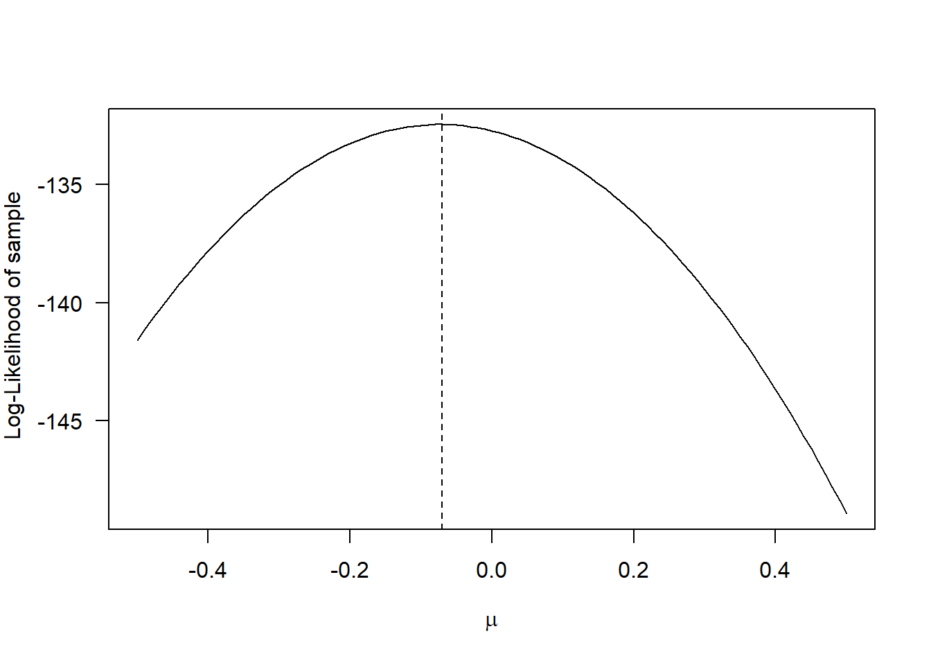
Although the shapes of the curves are different, the maximum occurs for the same value of \(\mu\). Note that there is nothing special about the natural logarithm: we could have taken the logarithm with base 10 or any other base. But it is customary to use the natural logarithm as some important probability density functions are exponential functions (e.g. the Normal distribution, see above), so taking the natural logarithm makes mathematical analyses easier.

You may have noticed that the optimal value of \(\mu\) was not exactly 0, even though the data was generated from a Normal distribution with \(\mu\) = 0. This is the reason why it is called a maximum likelihood estimator. The source of such deviation is that the sample is not a perfect representation of the population, precisely because of the randomness in the sampling procedure. A nice property of MLE is that, generally, the estimator will converge asymptotically to the true value in the population (i.e. as sample size grows, the difference between the estimate and the true value decreases).

The final technical detail you need to know is that, except for trivial models, the MLE method cannot be applied analytically. One option is to try a sequence of values and look for the one that yields maximum log-likelihood (this is known as grid approach as it is what I tried above). However, if there are many parameters to be estimated, this approach will be too inefficient. For example, if we only try 20 values per parameter and we have 5 parameters we will need to test 3.2 million combinations.

Instead, the MLE method is generally applied using algorithms known as non-linear optimizers. You can feed these algorithms any function that takes numbers as inputs and returns a number as ouput and they will calculate the input values that minimize or maximize the output. It really does not matter how complex or simple the function is, as they will treat it as a black box. By convention, non-linear optimizers will minimize the function and, in some cases, we do not have the option to tell them to maximize it. Therefore, the convention is to minimize the negative log-likelihood (NLL).

Enough with the theory. Let’s estimate the values of \(\mu\) and \(\sigma\) from the first sample we generated above. First, we need to create a function to calculate NLL. It is good practice to follow some template for generating these functions. An NLL function should take two inputs: (i) a vector of parameter values that the optimization algorithm wants to test (pars) and (ii) the data for which the NLL is calculated. For the problem of estimating \(\mu\) and \(\sigma\), the function looks like this:

NLL = function(pars, data) {
  # Extract parameters from the vector
  mu = pars[1]
  sigma = pars[2]
  # Calculate Negative Log-LIkelihood
  -sum(dnorm(x = data, mean = mu, sd = sigma, log = TRUE))
}

The function dnorm returns the probability density of the data assuming a Normal distribution with given mean and standard deviation (mean and sd). The argument log = TRUE tells R to calculate the logarithm of the probability density. Then we just need to add up all these values (that yields the log-likelihood as shown before) and switch the sign to get the NLL.

We can now minimize the NLL using the function optim. This function needs the initial values for each parameter (par), the function calculating NLL (fn) and arguments that will be passed to the objective function (in our example, that will be data). We can also tune some settings with the control argument. I recommend to set the setting parscale to the absolute initial values (assuming none of the initial values are 0). This setting determines the scale of the values you expect for each parameter and it helps the algorithm find the right solution. The optim function will return an object that holds all the relevant information and, to extract the optimal values for the parameters, you need to access the field par:

mle = optim(par = c(mu = 0.2, sigma = 1.5), fn = NLL, data = sample,
            control = list(parscale = c(mu = 0.2, sigma = 1.5)))
mle$par

##          mu       sigma 
## -0.07332745  0.90086176

It turns out that this problem has an analytical solution, such that the MLE values for \(\mu\) and \(\sigma\) from the Normal distribution can also be calculated directly as:

c(mu = mean(sample), sigma = sd(sample))

##         mu      sigma 
## -0.0733340  0.9054535

There is always a bit of numerical error when using optim, but it did find values that were very close to the analytical ones. Take into account that many MLE problems (like the one in the section below) cannot be solved analytically, so in general you will need to use numerical optimization.

MLE applied to a scientific model

In this case, we have a scientific model describing a particular phenomenon and we want to estimate the parameters of this model from data using the MLE method. As an example, we will use a growth curve typical in plant ecology.

Let’s imagine that we have made a series of a visits to a crop field during its growing season. At every visit, we record the days since the crop was sown and the fraction of ground area that is covered by the plants. This is known as ground cover (\(G\)) and it can vary from 0 (no plants present) to 1 (field completely covered by plants). An example of such data would be the following (data belongs to my colleague Ali El-Hakeem):

data = data.frame(t = c(0, 16, 22, 29, 36, 58),
                  G = c(0, 0.12, 0.32, 0.6, 0.79, 1))
plot(data, las = 1, xlab = "Days after sowing", ylab = "Ground cover")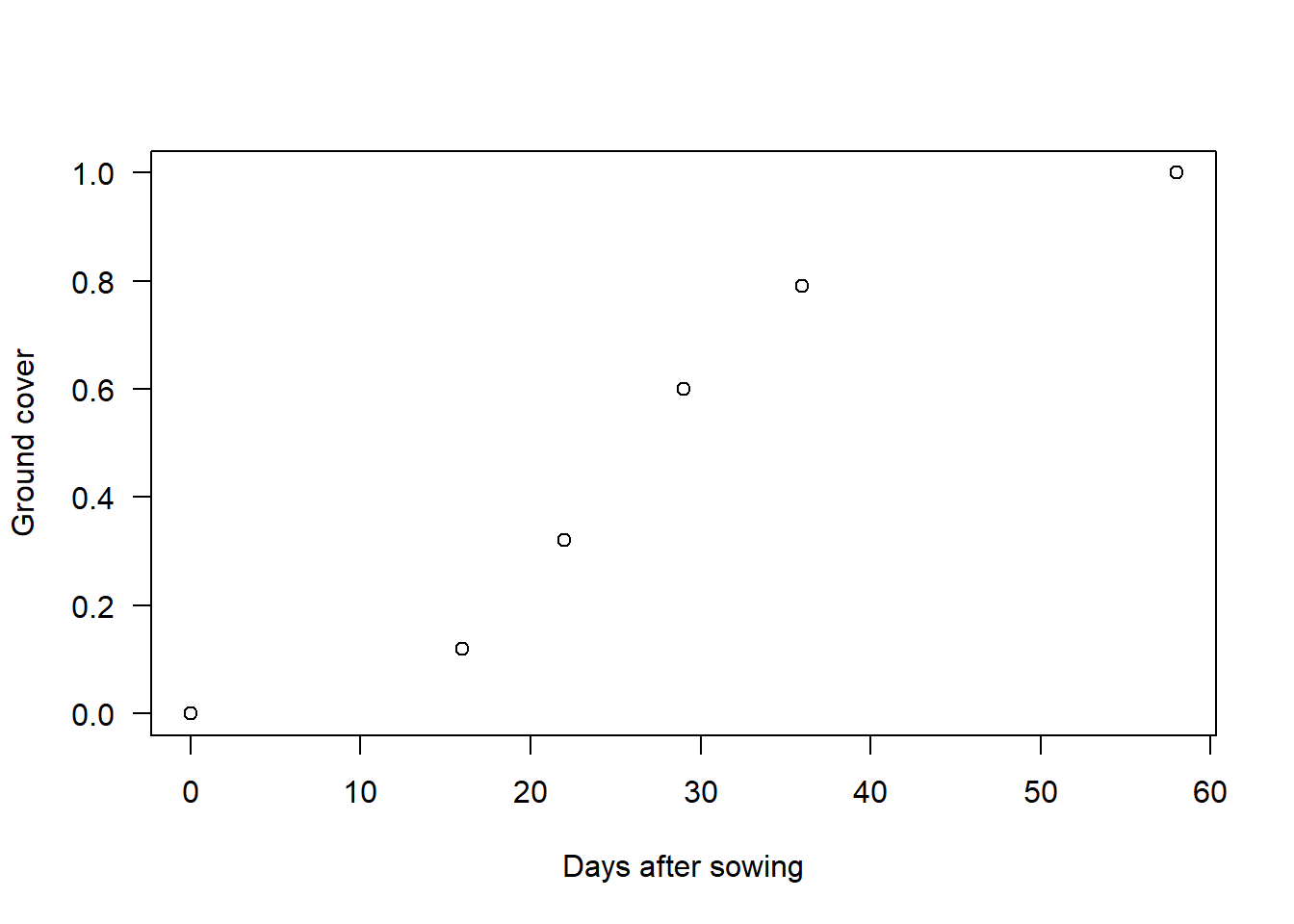

Our first intuition would be to use the classic logistic growth function (see here) to describe this data. However, this function does not guarantee that \(G\) is 0 at \(t = 0\) . Therefore, we will use a modified version of the logistic function that guarantees \(G = 0\) at \(t = 0\) (I skip the derivation):

\[ G = \frac{\Delta G}{1 + e^{k \left(t - t_{h} \right)}} - G_{o} \]

where \(k\) is a parameter that determines the shape of the curve, \(t_{h}\) is the time at which \(G\) is equal to half of its maximum value and \(\Delta G\) and \(G_o\) are parameters that ensure \(G = 0\) at \(t = 0\) and that \(G\) reaches a maximum value of \(G_{max}\) asymptotically. The values of \(\Delta G\) and \(G_o\) can be calculated as:

\[ \begin{align} G_o &= \frac{\Delta G}{1 + e^{k \cdot t_{h}}} \\ \Delta G &= \frac{G_{max}}{1 - 1/\left(1 + e^{k \cdot t_h}\right)} \end{align} \]

Note that the new function still depends on only 3 parameters: \(G_{max}\), \(t_h\) and \(k\). The R implementation as a function is straightforward:

G = function(pars, t) {
  # Extract parameters of the model
  Gmax = pars[1]
  k = pars[2]
  th = pars[3]
  # Prediction of the model
  DG = Gmax/(1 - 1/(1 + exp(k*th)))
  Go = DG/(1 + exp(k*th))
  DG/(1 + exp(-k*(t - th))) - Go
}

Note that rather than passing the 3 parameters of the curve as separate arguments I packed them into a vector called pars. This follows the same template as for the NLL function described above.

Non-linear optimization algorithms always requires some initial values for the parameters being optimized. For simple models such as this one we can just try out different values and plot them on top of the data. For this model, \(G_{max}\) is very easy as you can just see it from the data. \(t_h\) is a bit more difficult but you can eyeball it by cheking where \(G\) is around half of \(G_{max}\). Finally, the \(k\) parameter has no intuitive interpretation, so you just need to try a couple of values until the curve looks reasonable. This is what I got after a couple of tries:

plot(data, las = 1, xlab = "Days after sowing", ylab = "Ground cover")
curve(G(c(Gmax = 1, k = 0.15, th = 30), x), 0, 60, add = TRUE)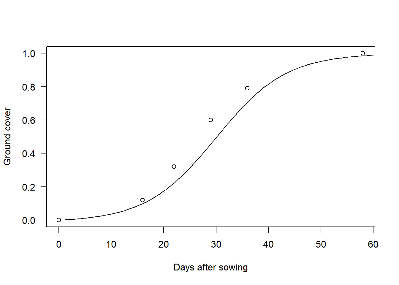

If we want to estimate the values of \(G_{max}\), \(k\) and \(t_h\) according to the MLE method, we need to construct a function in R that calculates NLL given an statistical model and a choice of parameter values. This means that we need to decide on a distribution to represent deviations between the model and the data. The canonical way to do this is to assume a Normal distribution, where \(\mu\) is computed by the scientific model of interest, letting \(\sigma\) represent the degree of scatter of the data around the mean trend. To keep things simple, I will follow this approach now (but take a look at the final remarks at the end of the article). The NLL function looks similar to the one before, but now the mean is set to the predictions of the model:

NLL = function(pars, data) {
  # Values predicted by the model
  Gpred = G(pars, data$t)
  # Negative log-likelihood 
  -sum(dnorm(x = data$G, mean = Gpred, sd = pars[4], log = TRUE))
}

We can now calculate the optimal values using optim and the “eyeballed” initial values (of course, we also need to have an initial estimate for \(\sigma\)):

par0 = c(Gmax = 1.0, k = 0.15, th = 30, sd = 0.01)
fit = optim(par = par0, fn = NLL, data = data, control = list(parscale = abs(par0)), 
            hessian = TRUE)
fit$par

##        Gmax           k          th          sd 
##  0.99926603  0.15879585 26.70700004  0.01482376

Notice that eyeballing the initial values already got us prettly close to the optimal solution. Of course, for complicated models your initial estimates will not be as good, but it always pays off to play around with the model before going into optimization. Finally, we can compare the predictions of the model with the data:

plot(data, las = 1, xlab = "Days after sowing", ylab = "Ground cover")
curve(G(fit$par, x), 0, 60, add = TRUE)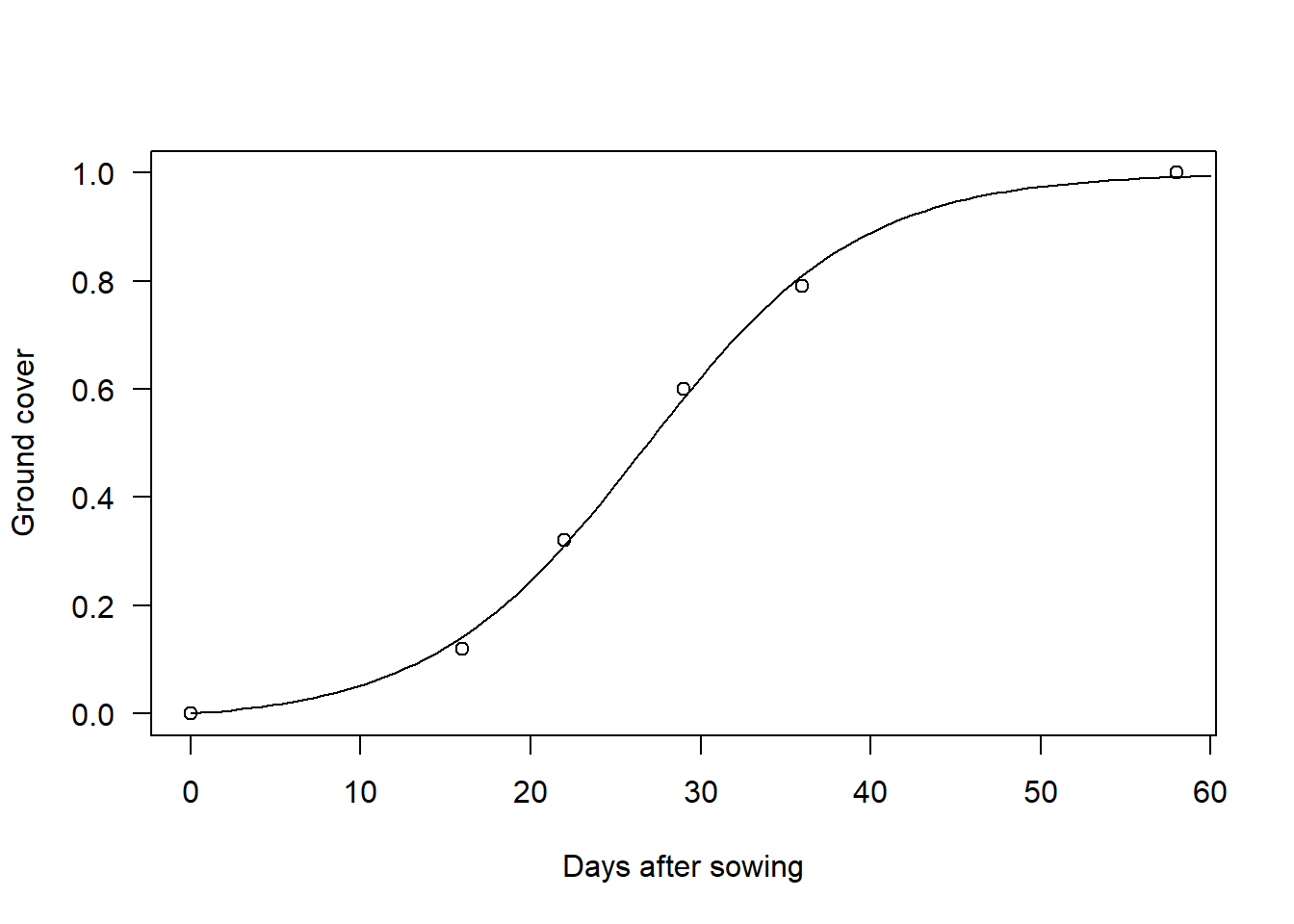

Final remarks

The model above could have been fitted using the method of ordinary least squares (OLS) with the R function nls. Actually, unless something went wrong in the optimization you should obtain the same results as with the method described here. The reason is that OLS is equivalent to MLE with a Normal distribution and constant standard deviation. However, I believe it is worthwhile to learn MLE because:

• You do not have to restrict yourself to the Normal distribution. In some cases (e.g. when modelling count data) it does not make sense to assume a Normal distribution. Actually, in the ground cover model, since the values of \(G\) are constrained to be between 0 and 1, it would have been more correct to use another distribution, such as the Beta distribution (however, for this particular data, you will get very similar results so I decided to keep things simple and familiar).

• You do not have to restrict yourself to modelling the mean of the distribution only. For example, if you have reason to believe that errors do not have a constant variance, you can also model the \(\sigma\) parameter of the Normal distribution. That is, you can model any parameter of any distribution.

• If you undestand MLE then it becomes much easier to understand more advanced methods such as penalized likelihood (aka regularized regression) and Bayesian approaches, as these are also based on the concept of likelihood.

• You can combine the NLL of multiple datasets inside the NLL function, whereas in ordinary least squares, if you want to combine data from different experiments, you have to correct for different in scales or units of measurement and for differences in the magnitude of errors your model makes for different datasets.

• Many methods of model selection (so-called information criteria such as AIC) are based on MLE.

• Using a function to compute NLL allows you to work with any model (as long as you can calculate a probability density) and dataset, but I am not sure this is possible or convenient with the formula interface of nls (e.g combining multiple datasets is not easy when using a formula interface).

Of course, if none of the above applies to your case, you may just use nls. But at least now you understand what is happening behind the scenes. In future posts I discuss some of the special cases I gave in this list. Stay tuned!