Estimating variance: should I use n or n - 1? The answer is not what you think

Estimates of population parameters based on samples are not exact: there is always some error involved. In principle, one can estimate a population parameter with any estimator, but some will be better than others. There is one particular case which was always very confusing to me (because of the multiple alternatives) and that is the estimation of the variance of a Normal population from a sample. In this article I describe the properties and tradeoffs among the different alternatives and discuss how important these differences are.

Let’s first get the basic concepts right. The variance of any random variable x is formally defined as the “expected value of the squared deviation from the mean of x”. If x is described by a particular distribution, then the variance will be a function of the parameters of that distribution. For every distribution, there is a formula to calculate its variance which you can derive with calculus (or you can check the Wikipedia page for that distribution). However, I prefer to focus on the variance of a sample, because (i) you can always generate a sample from any distribution and estimate its variance from it and (ii) most of the time we are dealing with samples of data anyways. By definition, the variance of a random sample (X) is the average squared distance from the sample mean (\(\bar{x}\)), that is:

\[ \text{Var}(\textbf{X}) = \frac{\sum_{i=1}^{i=n}\left(x_i - \bar{x} \right)^2}{n} \]

Now, one of the things I did in the last post was to estimate the parameter \(\sigma\) of a Normal distribution from a sample (the variance of a Normal distribution is just \(\sigma^2\)). The MLE estimator for \(\sigma^2\) can be derived analytically and coincides with the variance of the sample (i.e. the formula I show above). However, I am sure you have come across an alternative estimator for \(\sigma^2\) that uses n - 1 rather than n:

\[ \text{AltVar}(\textbf{X}) = \frac{\sum_{i=1}^{i=n}\left(x_i - \bar{x} \right)^2}{n - 1} \]

The fact that this is often called the “sample variance” is really confusing because this formula does not follow the definition of variance for a random variable (i.e. it is not the “expected value of the squared deviation from the mean”). The reason you may have read or been told to use this alternative rather than the original one is because this alternative estimator is unbiased while the original one is not. That sounds like a good thing. No one wants to be biased, right? But, what does it mean to be unbiased and should we care about it?

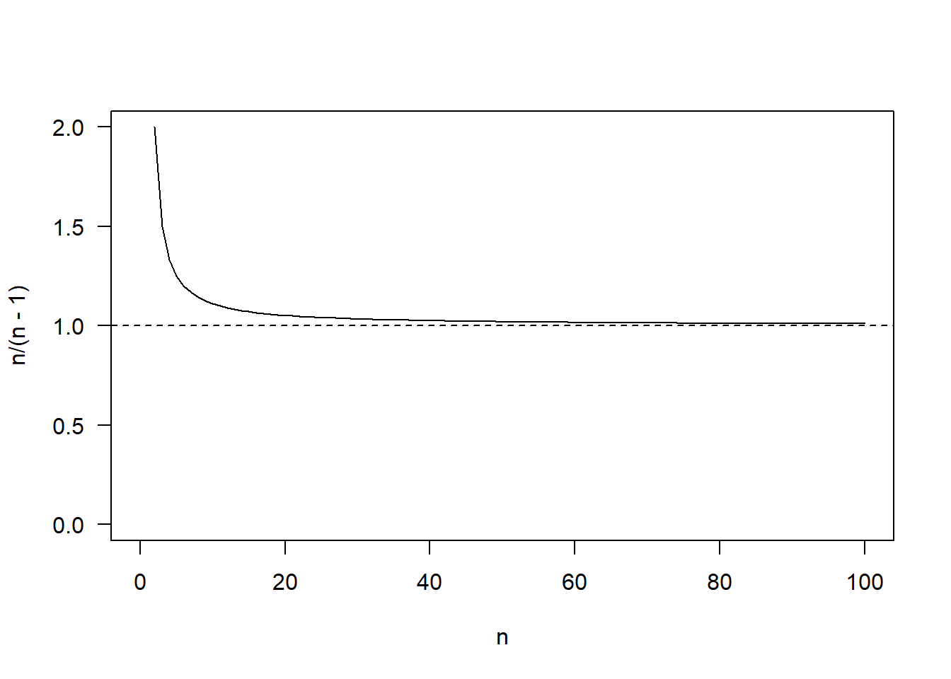
Before that, it is important to remember that if the sample is large, it does not really matter which estimator you use, because the ratio n/(n - 1) converges towards 1. This means that both estimators are asymptotically unbiased:

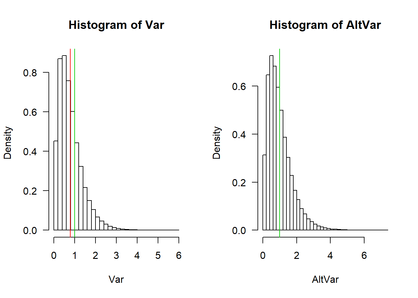
Being unbiased for any sample size means that the average of the sampling distribution of the estimator is equal to the true value of the parameter being estimated. Let’s check that out with a simulation. If we generate a hundred thousand samples of size 5 from a standard Normal distribution (\(\mu\) = 0, \(\sigma\) = 1) and we construct the sampling distribution of the original and alternative variance estimators, we get the following:

library(furrr)
plan(multiprocess)
N = 1e5
n = 5
samples = future_map_dfc(1:N, ~rnorm(n))
Var = future_map_dbl(samples, ~sum((.x - mean(.x))^2)/n)
AltVar = future_map_dbl(samples, ~sum((.x - mean(.x))^2)/(n - 1))
par(mfrow = c(1,2))
hist(Var, breaks = 30, prob = TRUE, las = 1)
abline(v = c(mean(Var), 1), col = c(2,3))
hist(AltVar, breaks = 30, prob = TRUE, las = 1)
abline(v = c(mean(AltVar), 1), col = c(2,3))

These are the sampling distributions of the two estimators. The green lines represents the true value (\(\sigma^2 = 1\)) whereas the red lines are the means of each sampling distribution. The two sampling distributions look very similar but in the case of the original formula for the variance there is a difference between the true value and the mean of the sampling distribution (i.e. the red and green lines do not coincide). This difference is called bias, which we can easily calculate:

bias_Var = mean(Var) - 1
bias_AltVar = mean(AltVar) - 1
c(bias_Var, bias_AltVar)

## [1] -0.201394170 -0.001742713

You can see that the bias of the alternative variance estimator is 100 times smaller (theoretically it should be 0, but there is always some numerical error in a Monte Carlo simulation). But does it really matter? Do we really care, in practice, about the average of estimates calculated from a hundred thousand independent samples? I mean, in most case we only have one sample, right? Note that the bias does not say anything about how far one sample is from the true value.

Instead, it sounds more reasonable to focus on measures of the average distance between an estimate and the true value (i.e. the average error of the estimator). The most common measure of error is the mean squared error between the estimates (\(\hat{\sigma^2}\)) and the true value (\(\sigma^2\)):

\[ \text{MSE} = \frac{\sum_{i=1}^{i=n}\left(\hat{\sigma}^2_i - \sigma^2 \right)^2}{n} \]

We can decomponse the mean squared error into the sum of two components:

\[ \text{MSE} = \text{Bias}^2 + \text{Variance} \]

That is, the mean squared error of an estimator is equal to the sum of the squared bias of the estimator (what we calculated before) and the variance of the estimator (i.e. how much the estimates vary from sample to sample). By using n - 1 instead of n we decreased the bias of the estimator, but what about the variance of the estimator? We can check this easily:

c(var(Var), var(AltVar))

## [1] 0.3183061 0.4973532

This is becoming a bit of a tongue twister, but hopefully you can see that I calculated the variance of the variance estimators (there is variance within a sample and this variance varies across samples…). We can see that the original formula for the variance leads to a lower variance than the alternative one. So what are the mean squared errors of the two alternatives?

MSE_Var = sum((Var - 1)^2)/N
MSE_AltVar = sum((AltVar - 1)^2)/N
c(MSE_Var, MSE_AltVar)

## [1] 0.3588625 0.4973513

So, the estimator with the original formula actually makes, on average, a smaller error than the alternative one. The reason is that the decrease in bias when using n - 1 does not offset the increase in variance that comes with it. This trade-off is common with parameter estimators (and with models too). It is known as the bias-variance tradeoff and it is a big topic in predictive modelling and machine learning. The idea is that a little bias can reduce the error of estimation if it also decreases substantially the variance of the estimator.

To see this bias-variance tradeoff in action, let’s generate a series of alternative estimators of the variance of the Normal population used above. The formula for each estimator will use a different correction term that is added to the sample size in the denominator (i.e. using n - 1 means a correction term of -1, whereas using n means a correction term of 0). For each estimator we calculate the bias, variance and mean squared error:

corr = -3:3
N = 1e5
n = 5
sampling_distros = matrix(NA, ncol = length(corr), nrow = N)
for(i in 1:length(corr)) {
  sampling_distros[,i] = future_map_dbl(samples, ~sum((.x - mean(.x))^2)/(n + corr[i]))
}
Bias = colMeans(sampling_distros) - 1
MSE = colMeans((sampling_distros - 1)^2)
Variance = MSE - Bias^2

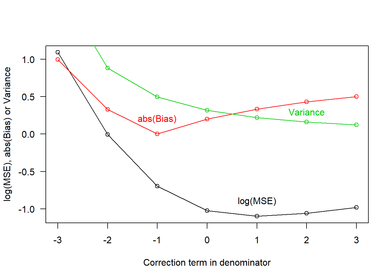
And if we plot the result you see that, indeed, the smallest bias occurs with a correction term of -1 and the (absolute) bias increases for any other correction term. On the other hand, the variance always decreases as the correction terms increases:

plot(corr, log(MSE), las = 1, t = "o", ylab = "log(MSE), abs(Bias) or Variance",
     xlab = "Correction term in denominator")
points(corr, abs(Bias), col = 2, t = "o")
points(corr, Variance, col = 3, t = "o")
text(c(1, -1, 2), y = c(-0.9, 0.2, 0.3), col = 1:3,
     labels = c("log(MSE)", "abs(Bias)", "Variance"))

The tradeoff means that the lowest MSE actually happens with a correction term of 1. That is, if you really want to minimize the mean squared error of your variance estimate for the Normal distribution, you should divide by n + 1 rather than n or n - 1!

Of course, we should ask ourselves, is the mean squared error what we want to minimize? What about mean absolute error? (you can try doing the calculations for this error measure as an exercise; I will tell you that the optimal correction term for this criterion is 0). My point is that, depending on the criterion that you use, one estimator will perform better than another but there is not consistency across criteria because of the bias-variance tradeoff.

The important thing to remember is that these are all estimates of an unknown quantity, so they are all wrong. It is perhaps more important to learn how to calculate the uncertainty in the estimate and deal with this uncertainty explicitly in any further analysis, rather than trying to optimize a particular criterion (unless you have very good reasons to use a specific criterion). The reason why maximum likelihood estimators are popular is because, although they may not be the optimal estimators for some criterion, they do well across the different criteria. In addition, maximum likelihood estimators are based on a simple principle and can be computed for any parameter of any model as long as you can calculate the negative log likelihood as shown in my previous post. This means that if you stick to a general principle like maximum likelihood, you will not need to remember dozens of estimators for different problems, which will make your life easier!